![]()
Quarantine plus Avatar on Netflix? I surrender!
My wife and I recently finished a beloved show that we each really enjoyed watching growing up - Avatar: The Last Airbender. Since its arrival on Netflix, I have spoken with a number of people who have once again fallen in love with this show from their childhood. To be honest, watching Avatar as an adult was probably even more enjoyable!
Instead of hiding my nerd-self from the world, I will embrace it here for all to see by combining my fondness for Avatar with my love of all things data and R. I hope you find this entertaining!
Also, if you don’t care about R code, but are just a fan of the show, scroll past the code and get to the insights!
Sadly, Aang never mastered databending
As always, we’ll install and/or load our needed packages, and read in our data.
# packages

# install.packages(c("tidyverse", "tidytext", "textdata, "DataExplorer", "devtools",
# "ggrepel", "wordcloud"))
# devtools::install_github('cttobin/ggthemr')
# devtools::install_github("averyrobbins1/sometools")
# devtools::install_github("averyrobbins1/appa")

library(tidyverse) # all the things
library(tidytext) # text analysis using tidy principles
library(ggrepel) # easy text labels for ggplot2 plots
#library(ggthemr) # nice ggplot2 themes
library(sometools) # my personal R package
library(glue) # run code inside of strings
library(gghighlight) # easily highlight data in a ggplot2
library(patchwork) # composing multiple ggplot2 plots
library(wordcloud) # make wordclouds

# set plot theme

#ggthemr('fresh')

# data

dat <- appa::appa

glimpse(dat)
Rows: 13,385
Columns: 12
$ id                <int> 1, 2, 3, 4, 5, 6, 7, 8, 9, 10, 11, 12, ...
$ book              <fct> Water, Water, Water, Water, Water, Wate...
$ book_num          <int> 1, 1, 1, 1, 1, 1, 1, 1, 1, 1, 1, 1, 1, ...
$ chapter           <fct> The Boy in the Iceberg, The Boy in the ...
$ chapter_num       <int> 1, 1, 1, 1, 1, 1, 1, 1, 1, 1, 1, 1, 1, ...
$ character         <chr> "Katara", "Scene Description", "Sokka",...
$ full_text         <chr> "Water. Earth. Fire. Air. My grandmothe...
$ character_words   <chr> "Water. Earth. Fire. Air. My grandmothe...
$ scene_description <list> [<>, <>, "[Close-up of the boy as he g...
$ writer            <chr> "<U+200E>Michael Dante DiMartino, Bryan Koniet...
$ director          <chr> "Dave Filoni", "Dave Filoni", "Dave Fil...
$ imdb_rating       <dbl> 8.1, 8.1, 8.1, 8.1, 8.1, 8.1, 8.1, 8.1,...
Wait… an R package named appa? Named after our favorite sky bison? That’s right. Having a lot of free time on a weekend means webscraping a bunch of Avatar data, tidying it up, and putting it in an R package. If you want access to the dataset used here, just install it from GitHub:
devtools::install_github("averyrobbins1/appa")
I will upload a post documenting the webscraping journey soon! But first, let’s answer some Avatar questions.
Imdb ratings
The best and the worst
The dataset from appa include imdb ratings for each chapter (epsiode). What were people’s favorite chapters? Let’s plot chapters with ratings, and label some of the best and worst.
dat_ratings <- dat %>%
    distinct(book, chapter_num, chapter, imdb_rating) %>%
    group_by(book) %>%
    mutate(
        best_worst = case_when(
            imdb_rating %in%
                (slice_max(., order_by = imdb_rating, n = 1) %>%
                pull(imdb_rating)) ~ "best",
            imdb_rating %in%
                (slice_min(., order_by = imdb_rating, n = 1) %>%
                pull(imdb_rating)) ~ "worst",
            TRUE                  ~ "mid"
        )
    ) %>%
    ungroup()

dat_ratings %>%
    ggplot(aes(x = chapter_num, y = imdb_rating)) +
    geom_point(aes(color = book), size = 2) +
    geom_text_repel(
        dat_ratings %>% filter(best_worst != "mid"),
        mapping = aes(label = chapter),
        seed = 1, size = 3.25, alpha = .75, force = 5,
        direction = "both") +
    facet_wrap(~ book) +
    labs(
        x = "Chapters",
        y = "Imdb Ratings",
        color = "Book",
        title = "What were the highest and lowest rated chapters in each book?") +
    scale_y_continuous(breaks = seq(from = 7, to = 10, by = .5))
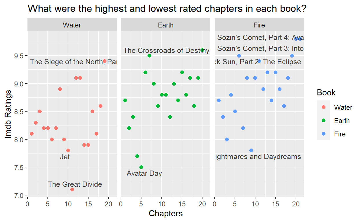
It’s kind of funny to see The Great Divide, Avatar Day, and Nightmares and Daydreams towards the lower end of the ratings. I remember each of those feeling sort of like “filler” episodes; they didnt’ contribute much to the main characters’ growth or the overall plot of the show. Also, its no surprise that most of the epic season finales were highly rated!
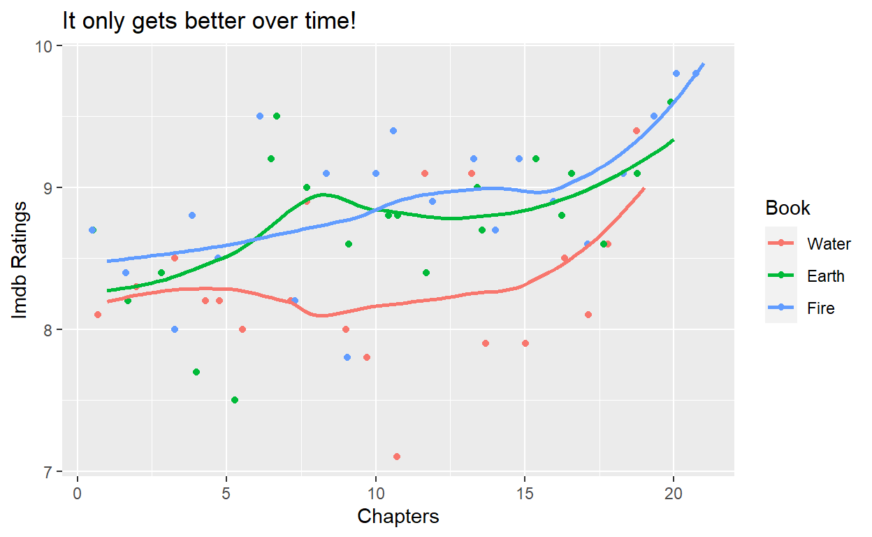
The Fire book was on fire
My wife and I also came to the consensus that book 3 was the best, followed by book 2. It seems that most people would agree.
dat_ratings %>%
    ggplot(aes(x = chapter_num, y = imdb_rating, color = book)) +
    geom_jitter(width = .5, height = 0) +
    geom_smooth(se = FALSE) +
    labs(
        x = "Chapters",
        y = "Imdb Ratings",
        color = "Book",
        title = "It only gets better over time!")
Transcripts
So far we have just been looking at imdb ratings, but most of the data that we have available are actually the transcripts. Let’s do some basic text analysis.
What are the most commonly spoken words by all the characters?
data("stop_words")

dat_tidy <- dat %>%
  select(book, chapter, chapter_num, character,
         character_words, imdb_rating) %>%
  filter(character != "Scene Description") %>%
  group_by(book) %>%
  mutate(line_num = row_number()) %>%
  ungroup() %>%
  unnest_tokens(word, character_words)

dat_tidy2 <- dat_tidy %>%
  anti_join(stop_words)

dat_tidy2 %>%
  count(word, sort = TRUE) %>%
  slice(1:20) %>%
  mutate(word = fct_reorder(word, n)) %>%
  ggplot(aes(x = n, y = word)) +
  geom_col() +
  geom_text(aes(label = n), nudge_x = 12) +
  labs(title = "Most common words spoken in Avatar: The Last Airbender",
       x = "Count",
       y = "Words Spoken") +
  gghighlight(word %in% c("fire", "appa", "uncle"))
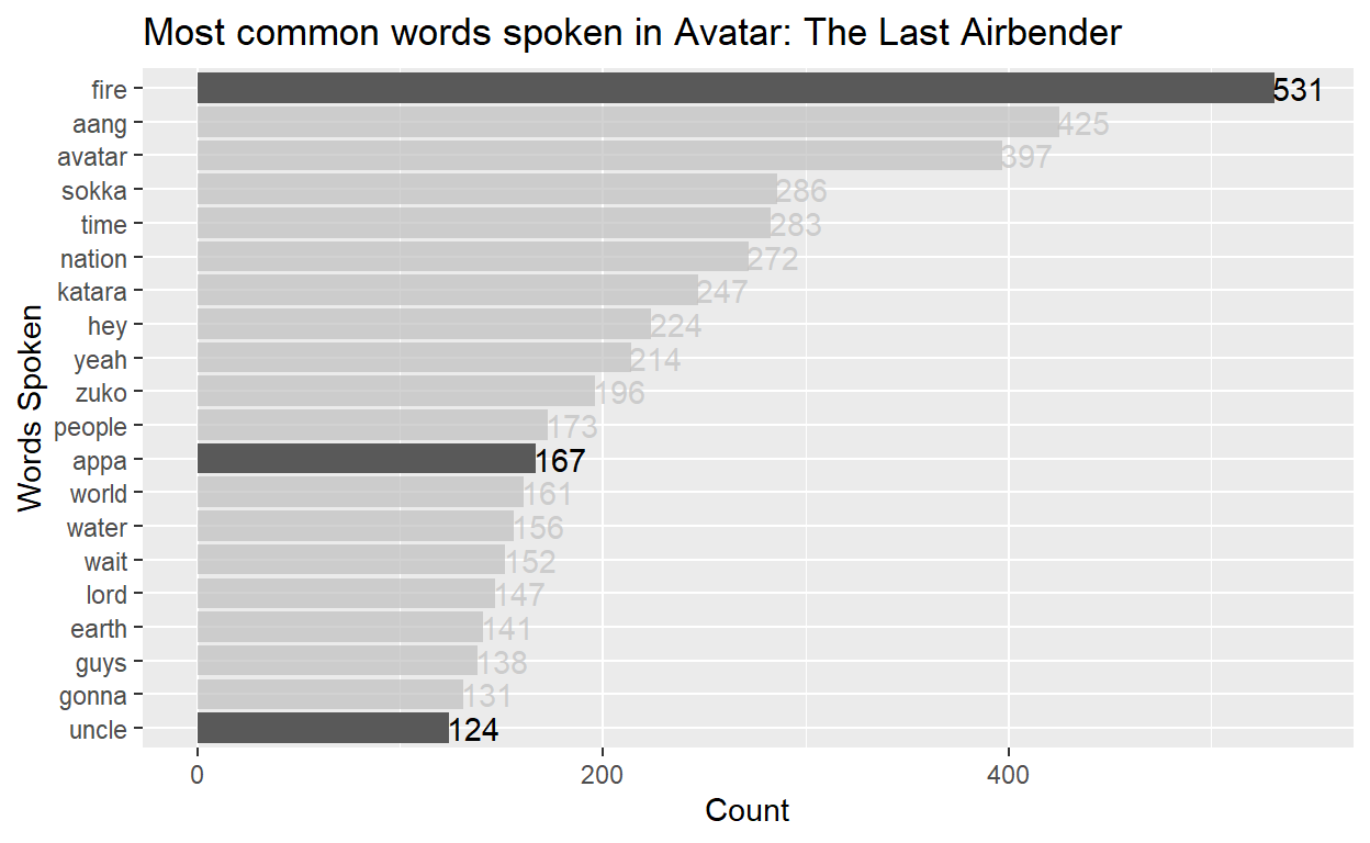
After filtering out all of the stop words, here are my first impressions:
It is significant that “fire” is the most spoken word in the series. Fire is symbolic of many things, including life and death. In the series especially, it is inseparably connected to the ultimate obstacle to world peace, the Fire Nation, and to Aang’s greatest foe, the Fire Lord.
My first thought as to the reason of the high occurence of the word appa: “Appa, yip, yip!”
Wow! I love that “uncle” made the top 20 most common words. Uncle Iroh is definitely one of my favorite characters. He is very wise and beloved by all.
I am curious to know if pretty much all of those mentions of “uncle” Iroh are from his nephew zuko. Let’s find out.
dat_tidy2 %>%
  filter(word == "uncle") %>%
  count(character, sort = TRUE) %>%
  slice(1:10) %>%
  mutate(character = fct_reorder(character, n)) %>%
  ggplot(aes(x = n, y = character)) +
  geom_col() +
  geom_text(aes(label = n), nudge_x = 1.5) +
  gghighlight(character == "Zuko") +
  labs(title = "Who said uncle?", x = "Word Count", y = "Characters")
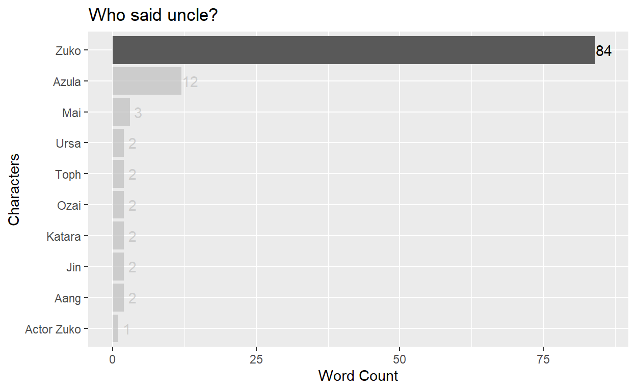
Well, that certainly checks out haha. Zuko was often with his uncle. This also makes me want to see all of the most common words of each of our favorite characters.
fav_characters <- c("Aang", "Katara", "Sokka", "Toph", "Iroh", "Zuko")

# let's make a quick helper function

top_words <- function(fav){
  character_plot <- dat_tidy2 %>%
  filter(character == fav) %>%
  count(word, sort = TRUE) %>%
  slice(1:10) %>%
  mutate(word = fct_reorder(word, n)) %>%
  ggplot(aes(x = n, y = word)) +
  geom_col() +
  geom_text(aes(label = n), size = 2.75, nudge_x = -4) +
  labs(title = glue("{fav}"), y = NULL, x = NULL)
}

plots <- map(fav_characters, top_words)

patched_plots <- patchwork::wrap_plots(plots)

words <- c("katara","aang","fire", "toes", "tea", "honor")

index <- 1:6

wrap_plots(
  map2(
    index, words, ~ patched_plots[[.x]] + gghighlight(word == .y)
    )
  ) + plot_annotation(title = "Most common words spoken by main characters")
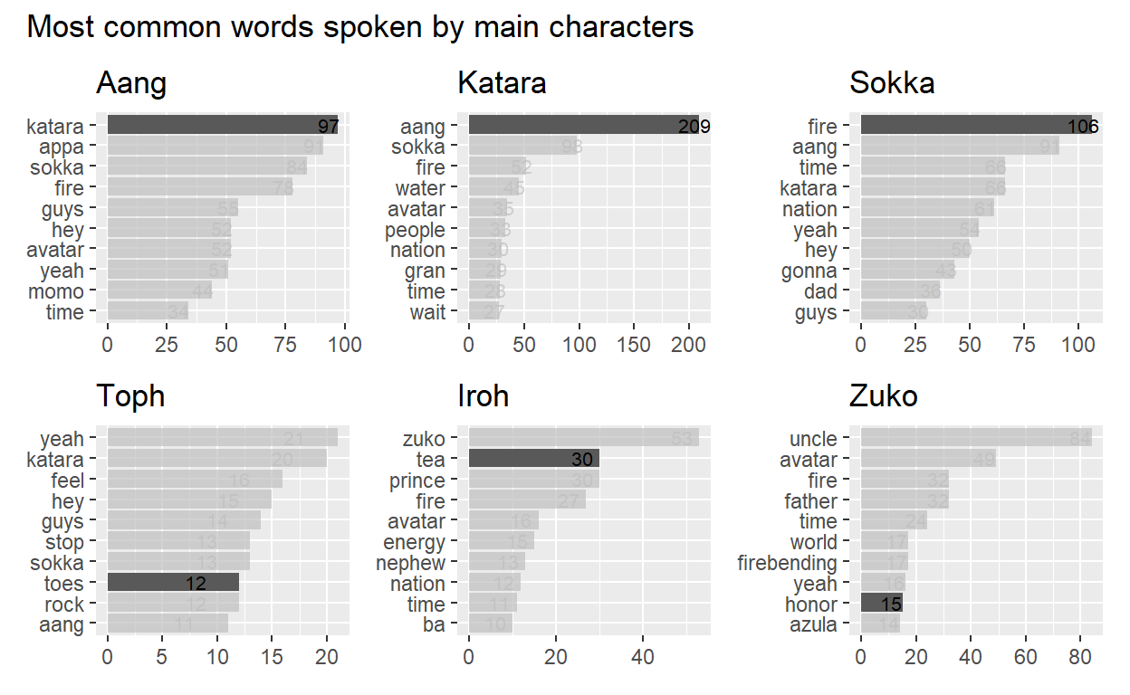
Well, Aang and Katara are certainly concerned with each other. Sokka was often focused on the war effort and the Fire Nation. Toph could see with her feet, and of course Iroh really loved his tea! Sadly, Zuko was just obsessed with his getting his honor from his father for the longest time.
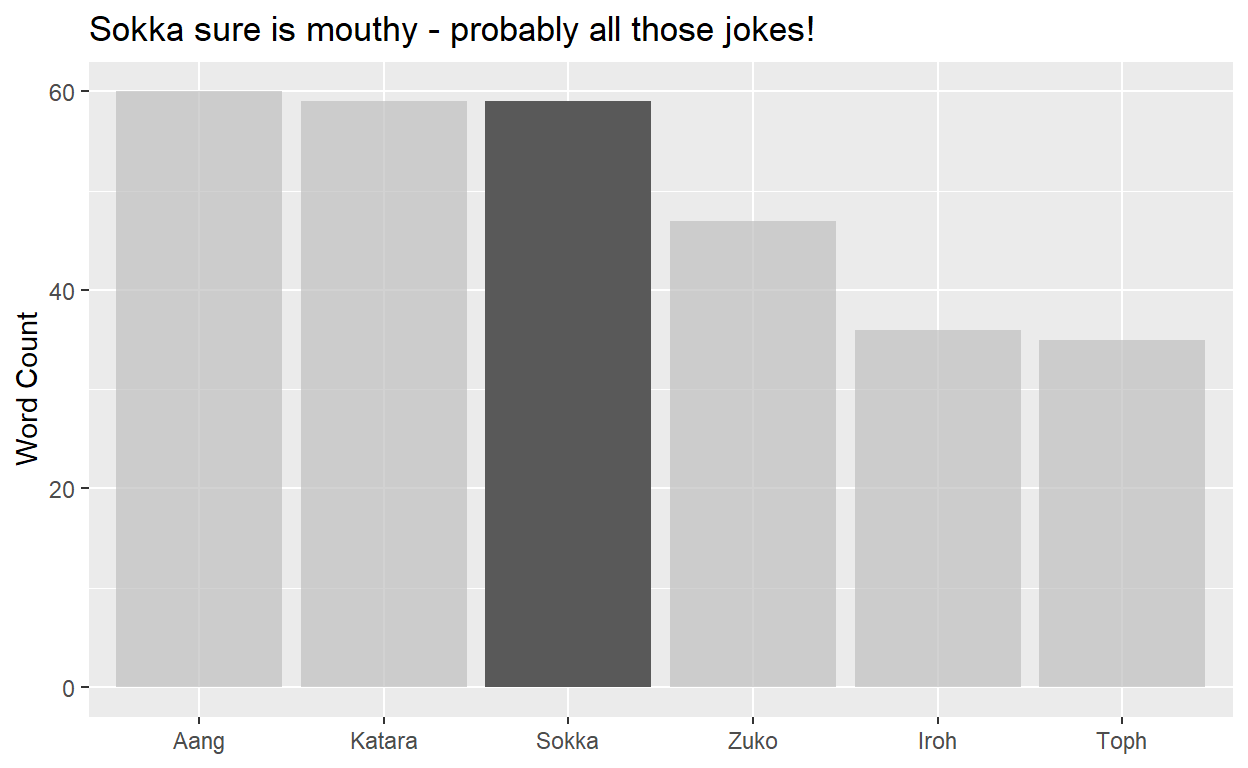
Let’s look more into the characters and how much they speak in general and in each episode. Note we are going back to the dataset including stop words.
dat_character_words <- dat_tidy %>%
  filter(character != "Scene Description") %>%
  count(chapter, chapter_num, character, imdb_rating) %>%
  add_count(character, wt = n, name = "word_count") %>%
  filter(word_count > 5000)

dat_character_words %>%
  count(character) %>%
  ggplot(aes(x = reorder(character, desc(n)) , y = n)) +
  geom_col() +
  labs(
    title = "Sokka sure is mouthy - probably all those jokes!",
    x = NULL, y = "Word Count"
  ) + gghighlight(character == "Sokka")
Let’s look into any relationships that may exist between certain characters speaking and episode ratings.
p1 <- dat_character_words %>%
  ggplot(aes(x = chapter_num, y = imdb_rating, color = character, size = n)) +
  geom_point() +
  facet_wrap(~ character) +
  labs(
    x = "Chapters", y = "Imdb Rating",
    size = "Word Count"
  ) + guides(color = FALSE)

p2 <- dat_character_words %>%
  ggplot(aes(x = n, y = imdb_rating, color = character)) +
  geom_point() +
  geom_smooth(se = FALSE) +
  facet_wrap(~ character) +
  labs(
    x = "Word Count", y = "Imdb Rating"
  ) + guides(color = FALSE)

p1 / p2 +
  plot_annotation(
    title = "Do specific character's word count seem to affect chapter ratings?")
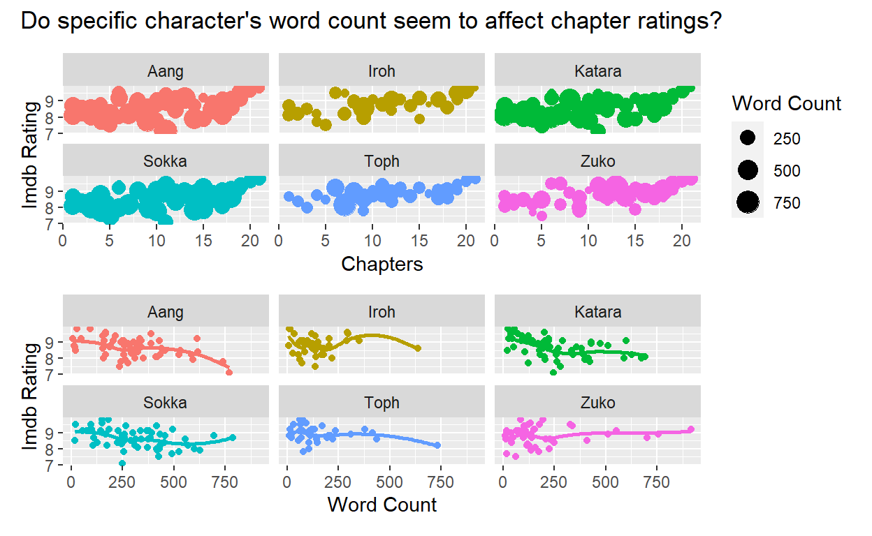
No crazy patterns jump out. There could be some slight linear relationships here, but we would want to run some models to get more certain results. This will suffice for now.
Quick sentiment analysis
Let’s use a sentiment lexicon (basically a dictionary to evaluate the emotion of a text) to get a feel for the tone of the show.
We’ll break each book up into segments of 50 lines each and analyze each segment. We’ll create a new column, sentiment, which is the difference between positive and negative word counts per segment. Also, let’s look at the entire transcript with and without the stop words.
dat_bing <- get_sentiments("bing")

dat_bing %>% head(3)
# A tibble: 3 x 2
  word     sentiment
  <chr>    <chr>
1 2-faces  negative
2 abnormal negative
3 abolish  negative
dat_sent <- dat_tidy %>% inner_join(dat_bing)
dat_sent_books <- dat_sent %>%
count(book, index = line_num %/% 50, sentiment) %>%
pivot_wider(names_from = sentiment, values_from = n) %>%
mutate(sentiment = positive - negative)
p3 <- dat_sent_books %>%
ggplot(aes(x = index, sentiment, fill = book)) +
geom_col(show.legend = FALSE) +
facet_wrap(~ book) +
labs(
title = "With stop words", y = "Sentiment", x = "Index"
)
dat_sent2 <- dat_tidy2 %>% inner_join(dat_bing)
dat_sent_books2 <- dat_sent2 %>%
count(book, index = line_num %/% 50, sentiment) %>%
pivot_wider(names_from = sentiment, values_from = n) %>%
mutate(sentiment = positive - negative)
p4 <- dat_sent_books2 %>%
ggplot(aes(x = index, sentiment, fill = book)) +
geom_col(show.legend = FALSE) +
facet_wrap(~ book) +
labs(
title = "Without stop words", y = "Sentiment", x = "Index"
)
p3 / p4
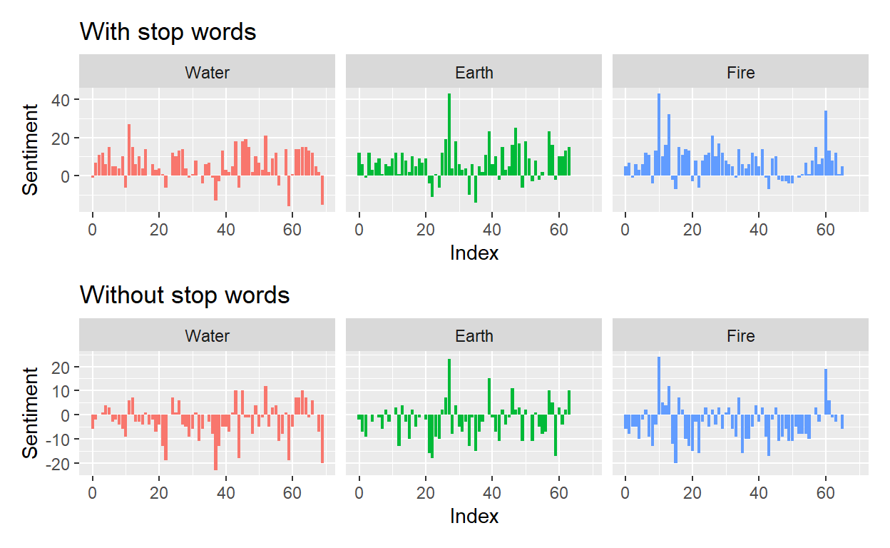
It looks like stop words are mostly positive, which doesn’t tell us much. I think the transcripts without the stop words would give greater insight into the overall sentiment of each book. When we look at segments without the stop words, the overall sentiment is negative. I would guess that that has to do with the whole 100 year war and everything. That being said, most people would argue that the message of Avatar: The Last Airbender is one of hope, friendship, and good overcoming evil.
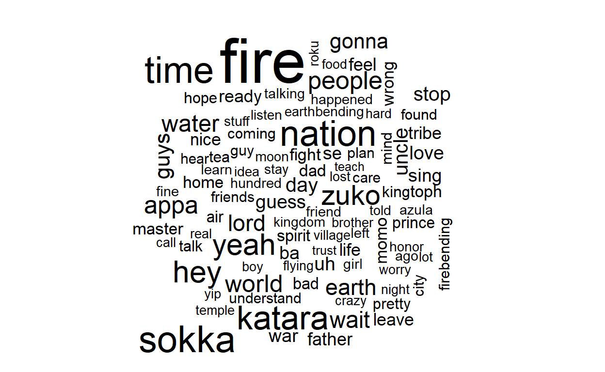
And a wordcloud just for fun
Conclusion
There is so much more potential here! This was honestly just the tip of the iceberg. I want to do more EDA, and I think it could be interesting to dive deeper into specific characters. Stayed tuned for more analysis and Avatar related fun in the future. Thanks for reading!